The general concept of a Bounding Volume Hierarchy (BVH) is to group or partition the space used by objects within it and wrap them up in a bounding box. The space is partitioned multiple times until each object in the scene has its own bounding box.
This is done because box intersection tests are computationally faster and cheaper than spherical (or other complex shape) intersection tests.
The construction of a BVH tree structure to be used by the raytracer was started by setting up the root node that should encompass all of the objects in the scene. This forms a bounding box around all of the objects. If a ray does not intersect with the root node then it means that no objects will need to be tested for intersections and the skybox colour will be returned for that pixel.
If a node’s bounding box still contains a significant number of objects (more than the leaf limit) then the node would be divided into two thus forming two child nodes. The divide should happen along the largest axis where one child will form a bounding box around all objects from one side of the divide while the other child will contain the remainder of the objects. When an node contains an object count of the leaf limit (4 in my case) or less, it will stop dividing that node and each object will have a bounding box placed around them and become a child of that node.
In raytracing we are looking for the nearest object that the ray hits – aka the object with the shortest distance from the ray’s origin. So how this is done with a BVH is by starting from the root node (top of the data structure) and traversing through each of its’ child nodes testing for intersections. If any intersection is found, you will test the children of that node. Whereas if no intersection was found for that node, you would skip all of it’s children as they are not in the intersection space. This has the potential to cut a significant number of tests from being performed.
An example of this is when a ray does not intersect with the root node then the entire tree is skipped and no further intersection tests are done for that ray. However if a ray passes through multiple objects, only the bounding boxes that contain those objects are tested, which means at least 1 to 4 (my leaf limit) leaf nodes are tested per bounding box will be tested for intersections.
If you had a 1024×1024 viewport, you would have a minimum of 1,048,576 rays cast out – each pixel having a ray cast from its position into the scene. Each ray will need to test if it hits an object in the scene and for that to be tested without any form of spatial partitioning, you will need to test each individual object. This becomes insanely inefficient when you think about it and if you have reflective materials and shadows being rendered, you will need to add additional rays to that when an intersection happens.
In my case, we have reflective materials and shadows being rendered. Reflections will bounce up to 4 times before hitting a recursion limit. The original unoptimised version of the raytracer performs 4,283,997,255 full sphere intersection tests and takes several (5 – 10) minutes to complete. The BVH optimised version performs 103,884,072 box intersection tests and 21,743,684 sphere intersection tests and takes approximately 500 ms to complete. The number of sphere intersection tests were reduced to 0.05076% of the original unoptimised amount. However if we were to add the cheaper box intersection tests then only 2.933% of the total number of intersection tests were performed.
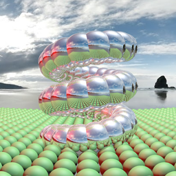
The first scene (the above image) contains around 950 spheres and went from taking several (5-10) minutes to approximately 500 ms to render the final image.
The second scene that we were given contains over 42000 spheres and went from 15 minutes with minor optimisations (multi-threading) to take approximately 800 – 900 ms to render.
The outcome that was learned throughout this learning exercise was that using a form of spatial partitioning will improve the performance of a ray tracing application if implemented correctly.
UPDATE: The second scene when unoptimised performs 173,005,702,902 sphere intersect tests. The BVH optimisations reduced that to 231,068,934 box intersect tests and only 40,043,462 sphere intersect tests.